Bernoulli vs binomial: one outcome or a count of trials

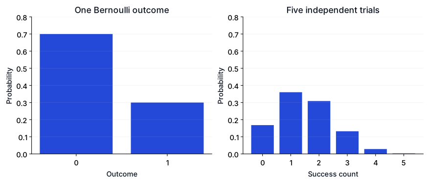
A Bernoulli variable represents one binary outcome, usually coded 0 or 1, with success probability p. A binomial variable counts successes across a fixed number n of independent Bernoulli trials with the same probability. The unit being modeled changes from one outcome to a count.

Suppose an invented practice exercise has probability 0.3 of being solved on a first attempt. Under a binomial model, five independent attempts on comparable exercises give a count K from 0 to 5. Calling them independent and equally difficult is part of the model, not something the word “binomial” establishes.

Calculate one probability by hand

For exactly two successes, there are C(5, 2) = 10 possible success positions. Each sequence has probability 0.3² × 0.7³. Multiplying gives P(K=2) = 0.3087.

The expected count is np = 1.5. The variance is np(1-p) = 1.05. For one Bernoulli outcome, the corresponding expectation is p and variance is p(1-p). A binomial distribution with n=1 therefore reduces to Bernoulli.

Compare the exact model with simulation

The simulation is synthetic and seeded. Its empirical frequency should be near the exact probability, but finite sampling does not promise identical values. The second construction makes all five outcomes share a single Bernoulli draw, deliberately breaking independence while preserving each trial's marginal success probability.

from math import comb
import numpy as np
n, p = 5, .3
probabilities = np.array([comb(n, k) * p**k * (1-p)**(n-k) for k in range(n+1)])
rng = np.random.default_rng(21)
independent = rng.binomial(1, p, size=(100000, n)).sum(axis=1)
shared = n * rng.binomial(1, p, size=100000)
print(f'exact P(K=2)={probabilities[2]:.4f}')
print(f'simulated P(K=2)={(independent == 2).mean():.4f}')
print(f'binomial mean={n*p:.2f} variance={n*p*(1-p):.2f}')
print(f'shared-cause variance={shared.var():.2f}')
print('shared-cause possible counts:', np.unique(shared).tolist())
assert np.isclose(probabilities.sum(), 1)
assert abs((independent == 2).mean() - probabilities[2]) < .01

Checked output:

exact P(K=2)=0.3087
simulated P(K=2)=0.3076
binomial mean=1.50 variance=1.05
shared-cause variance=5.24
shared-cause possible counts: [0, 5]

Diagnose the shared-cause failure

The dependent construction produces only 0 or 5 successes. Its variance is much larger than the independent binomial variance, even though each of the five component outcomes still has success probability 0.3. Marginal probabilities alone do not determine a sum's distribution; dependence matters.

In practice, repeated attempts can share a learner, machine, session or environment. Exercise difficulty may differ, and earlier attempts can influence later ones. These mechanisms can invalidate a simple binomial model. Do not treat thousands of correlated observations as thousands of independent trials merely because every outcome is binary.

If trial probabilities differ but outcomes remain independent, the count follows a different distribution, often called Poisson-binomial. If outcomes are dependent, the dependence structure also needs to be represented. Choosing an alternative requires understanding the data-generating process rather than selecting a distribution solely by its histogram.

Separate probability from estimation

Our p=0.3 is declared, not estimated. If you estimate p from a sample, the estimate has uncertainty. Using it in a binomial calculation does not make the resulting probability known exactly for future conditions.

Likewise, success is a label defined for a task, not necessarily a desirable outcome. A Bernoulli variable could indicate a failure, a defect or a completed exercise. State what 1 means before interpreting an average.

Extend the experiment

Increase n while keeping p fixed and compare the mean and spread. Then simulate two sets of five trials with probabilities 0.1 and 0.5 and inspect why pooling them changes the count distribution. Explain which assumptions hold before fitting a binomial model to the pooled records.

The Statistics course develops distributions and sampling. Review conditional probability for probability statements with different conditioning populations, and bootstrap confidence intervals for a separate approach to estimating uncertainty from sampled observations.

References

NumPy binomial generator — The binomial sampling API and its parameter interpretation.

SciPy binomial distribution — Probability mass function and distribution parameters.