Diffusion models step by step with a one-dimensional Gaussian

A diffusion model gradually adds noise to data and learns a reverse process that can generate samples. The forward arithmetic is easy to inspect in one dimension. A Gaussian teaching distribution also lets us calculate a reverse conditional exactly, revealing what a learned denoiser is trying to approximate without pretending that an analytic formula is a trained image model.

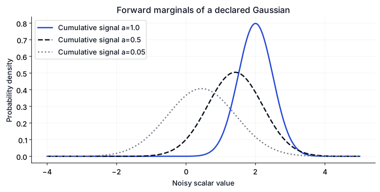
Our original data distribution is x0 ~ Normal(2, 0.5²). For cumulative signal coefficient a, define xt = sqrt(a) x0 + sqrt(1-a) epsilon, with independent standard Gaussian noise epsilon. As a decreases toward zero, the distribution approaches standard noise.

Derive the noisy mean and variance

The mean is sqrt(a) × 2. The variance is a × 0.25 + (1-a). Independence removes the covariance term. The standard deviation is the square root of that variance, not the variance itself.

At a=1, the original distribution is unchanged. Near a=0, the mean is near zero and the variance near one. These statements describe a marginal distribution across many examples; one noisy sample need not move monotonically toward zero.

Calculate the exact conditional for this special case

For an observed xt, Gaussian conditioning gives E[x0|xt] = mu + sqrt(a)*v/(a*v+1-a) × (xt-sqrt(a)*mu), where mu=2 and v=0.25. The conditional variance is v - a*v²/(a*v+1-a).

This posterior mean is a denoised estimate of the original scalar. A full diffusion sampler instead proceeds through a sequence of reverse transitions; the calculation below is not that entire sampler.

import numpy as np
mu, variance = 2., .25
rng = np.random.default_rng(46)
x0 = rng.normal(mu, np.sqrt(variance), 100000)
noise = rng.normal(size=len(x0))
for a in [1., .5, .05]:
    xt = np.sqrt(a)*x0 + np.sqrt(1-a)*noise
    expected_mean = np.sqrt(a)*mu
    expected_variance = a*variance + 1-a
    print(f'a={a:.2f} theoretical_mean={expected_mean:.3f}',
          f'theoretical_variance={expected_variance:.3f}',
          f'sample_mean={xt.mean():.3f} sample_variance={xt.var():.3f}')
    assert abs(xt.mean()-expected_mean) < .02
    assert abs(xt.var()-expected_variance) < .02
a, observed = .5, 0.
noisy_variance = a*variance + 1-a
gain = np.sqrt(a)*variance/noisy_variance
posterior_mean = mu + gain*(observed-np.sqrt(a)*mu)
posterior_variance = variance-a*variance**2/noisy_variance
print(f'given xt=0 at a=.5: posterior_mean={posterior_mean:.3f}',
      f'posterior_variance={posterior_variance:.3f}')
assert 0 < posterior_variance < variance

Checked output:

a=1.00 theoretical_mean=2.000 theoretical_variance=0.250 sample_mean=1.998 sample_variance=0.250
a=0.50 theoretical_mean=1.414 theoretical_variance=0.625 sample_mean=1.412 sample_variance=0.626
a=0.05 theoretical_mean=0.447 theoretical_variance=0.962 sample_mean=0.446 sample_variance=0.962
given xt=0 at a=.5: posterior_mean=1.600 posterior_variance=0.200

Explain what a learned denoiser adds

We can calculate this conditional because the original distribution is explicitly Gaussian with known parameters. Real image data does not offer such a convenient analytic density. A network is trained across noisy examples and timesteps to predict noise, the clean sample or another parameterization used by the chosen method.

The network does not simply subtract fresh random noise from an observed sample. It estimates a conditional quantity from noisy input and timestep information. The training objective, parameterization, variance schedule and sampler determine how those estimates enter reverse updates.

The posterior variance remains positive: one noisy observation does not uniquely identify its original value. Returning only the posterior mean gives a point estimate, not a sample from the full conditional. Confusing those operations can make a denoising demonstration appear to generate more diversity than it actually does.

Keep this scalar example in scope

No network is trained here, and no text-to-image capability is implied. The controlled evaluation checks that simulation agrees with the forward distribution's moments and that the analytic posterior has sensible variance. Image fidelity or prompt adherence requires a different dataset, model and evaluation task.

Extend the derivation

Choose another observed value and calculate the posterior before running the code. Then reduce a and inspect how the observation becomes less informative about x0. Finally, derive adjacent-step Gaussian transitions before attempting a multistep reverse sampler.

The Generative AI syllabus covers diffusion; lessons are being published. Review conditional probability for the conditioning idea and autoencoder reconstruction for a different representation-learning task that should not be conflated with diffusion sampling.

References

Denoising diffusion probabilistic models — Ho, Jain and Abbeel describe forward noising, learned reverse processes and the training connection.

NumPy normal sampling — Normal-distribution simulation used to check the declared arithmetic.