Gradient descent learning rates: convergence, oscillation and divergence

A gradient descent learning rate controls how far parameters move after each gradient calculation. On a quadratic, we can derive the boundary between convergence and instability, then verify it with a controlled experiment. This gives a firmer explanation than treating every oscillating loss curve as random bad luck.

Consider f(x, y) = (x² + 20y²) / 2, starting at (4, 1). Its gradient is (x, 20y). The two axes have different curvature: the second coordinate reacts twenty times as strongly to the same displacement.

Derive the update before plotting it

With learning rate eta, the next coordinates are x_next = (1 - eta)x and y_next = (1 - 20eta)y. Convergence requires both multipliers to have absolute value less than one. For this objective, that means 0 < eta < 0.1.

At eta = 0.1, the y multiplier is -1: the coordinate changes sign but never shrinks. A rate of 0.11 gives -1.2, so the magnitude grows. The x coordinate may still improve while the total objective diverges. Looking at a single parameter can conceal this failure.

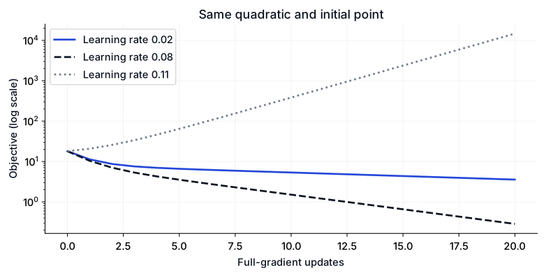
The plot uses the exact same objective, start and update rule as the script. Every method gets twenty full-gradient updates. No wall-clock or general optimizer ranking is inferred from this calculation.

Run the controlled experiment

import numpy as np

def objective(point):
    return (point[0] ** 2 + 20 * point[1] ** 2) / 2

for rate in [0.02, 0.08, 0.11]:
    point = np.array([4., 1.])
    history = [objective(point)]
    for _ in range(20):
        point -= rate * np.array([point[0], 20 * point[1]])
        history.append(objective(point))
    print(f'eta={rate:.2f} start={history[0]:.4f} end={history[-1]:.4f}',
          f'y_multiplier={1-20*rate:.2f}')
    assert np.isfinite(history).all()
    if rate < .1:
        assert history[-1] < history[0]
    else:
        assert history[-1] > history[0]

Checked output:

eta=0.02 start=18.0000 end=3.5656 y_multiplier=0.60
eta=0.08 start=18.0000 end=0.2848 y_multiplier=-0.60
eta=0.11 start=18.0000 end=14697.7913 y_multiplier=-1.20

Explain why the smaller rate can be slower

A rate of 0.02 is stable, but its x multiplier is 0.98, so progress along the flatter axis is slow. At 0.08, the x multiplier is 0.92 and the y multiplier is -0.6. The second coordinate oscillates while shrinking, and the final objective is lower after the same update budget.

Oscillation alone does not prove divergence. Check whether amplitudes or objective values shrink. Conversely, a few initially improving steps do not prove that a run will remain stable, especially when different directions have different curvature.

Feature scaling can reduce differences in curvature for some models. It does not make every loss convex, guarantee a single optimum or remove the need to choose an optimizer. See scaling versus normalization for the distinct data transformations involved.

Know what the stability bound assumes

The bound here applies to a fixed-rate, full-gradient update on this particular positive-definite quadratic. A general smooth convex objective requires its own curvature bound. Stochastic gradients, momentum, adaptive methods, changing schedules and nonconvex neural networks alter the dynamics.

A logarithmic objective axis helps compare orders of magnitude, but cannot display zero. The plotted values remain positive in our finite run. When diagnosing a real loss, also check for nonfinite values, broken gradients and a mismatch between the reported loss and the one being differentiated.

Extend the experiment

Add the boundary value 0.1 and verify that the y contribution remains constant. Then change the coefficient 20 to 100 and derive the new upper bound before running the code. Finally, rescale the second coordinate and compare the resulting curvature, keeping the objective interpretation explicit.

The Maths course connects gradients, geometry and optimization. First verify the squared-error derivative, then compare Adam and momentum SGD to see how optimizer state changes a related experiment.

References

Convex optimization lectures — Boyd and Vandenberghe provide the mathematical context for gradient methods and curvature bounds.