ROC AUC vs PR AUC: inspect what changes with class balance

ROC curves plot true-positive rate against false-positive rate as the score threshold changes. Precision-recall curves plot precision against recall. They summarize different aspects of a ranking, so a useful ROC AUC does not guarantee that the predicted-positive set has useful precision at an operational threshold.

The distinction becomes especially important when positive cases are rare. We will calculate three ranking summaries on invented scores, then duplicate negative cases to isolate the effect of class balance. This is an arithmetic demonstration, not a model benchmark or a claim about a real application.

Inspect the ranking before summarizing it

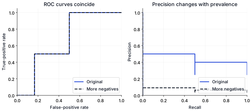
Our eight records are already ordered from highest to lowest score. Positive cases are at ranks 2 and 5. If we select the top two, one of two selected cases is positive: precision is 0.5 and recall is 0.5. At the top five, both positives are found: precision is 0.4 and recall is 1.

Average precision weights precision values by increments in recall. With these two positives and no tied positive scores, the calculation is (0.5 + 0.4) / 2 = 0.45. It is not automatically equal to the trapezoidal area under a plotted precision-recall curve.

import numpy as np
from sklearn.metrics import (
    average_precision_score, auc, precision_recall_curve, roc_auc_score,
)

y = np.array([0, 1, 0, 0, 1, 0, 0, 0])
scores = np.array([0.9, 0.8, 0.7, 0.6, 0.5, 0.4, 0.3, 0.2])

def report(name, labels, values):
    precision, recall, _ = precision_recall_curve(labels, values)
    print(name,
          f"prevalence={labels.mean():.3f}",
          f"ROC_AUC={roc_auc_score(labels, values):.3f}",
          f"AP={average_precision_score(labels, values):.3f}",
          f"trapezoid_PR={auc(recall, precision):.3f}")

report("original", y, scores)
# Make ten copies of every negative in total, preserving their score distribution.
expanded_y = np.concatenate([y, np.repeat(y[y == 0], 9)])
expanded_scores = np.concatenate([scores, np.repeat(scores[y == 0], 9)])
report("more_negatives", expanded_y, expanded_scores)
assert np.isclose(roc_auc_score(y, scores),
                  roc_auc_score(expanded_y, expanded_scores))

Expected output:

original prevalence=0.250 ROC_AUC=0.667 AP=0.450 trapezoid_PR=0.287
more_negatives prevalence=0.032 ROC_AUC=0.667 AP=0.077 trapezoid_PR=0.046

The printed trapezoidal result uses three-decimal floating-point formatting. Inspect full-precision values when comparing implementations rather than relying on rounding at the last displayed digit.

Explain the prevalence experiment

Each negative score has the same relative frequency within the negative class after duplication. The positive scores are unchanged. The true-positive and false-positive rates at each distinct threshold therefore stay the same, preserving the ROC curve and its area.

Precision has a different denominator: true positives divided by all predicted positives. More negatives at the same thresholds produce more false positives relative to the unchanged positive count. Precision and the PR summaries decrease.

This does not mean duplicating a dataset is a valid way to collect new evidence. It is a controlled construction for understanding a metric. Real distribution changes can also alter class-conditional scores, and then ROC AUC can change too.

Name the PR summary precisely

“PR AUC” is often used loosely. In this example, average precision and trapezoidal PR area differ substantially because they interpolate and summarize the curve differently. State the actual implementation and settings. For multiclass or multilabel tasks, also specify the positive class, averaging scheme and any weights.

The scikit-learn metric guide distinguishes average precision from trapezoidal integration. Reproducing the exact metric definition is necessary before comparing a reported result with another experiment.

Choose an operating point as well

Neither area tells you what will happen at the threshold your application uses. Inspect counts, precision, recall and the costs of errors at a candidate operating point. If a team can review only a fixed number of cases, precision or recall at that review budget may be closer to the actual decision.

Threshold selection belongs inside the development process. Do not repeatedly tune the threshold on the final held-out test. AUC also measures ranking rather than probability calibration: a score can order cases well while giving poorly calibrated numerical probabilities.

Extend the example

Swap the two highest scores and observe which summaries change. Then introduce a tie between a positive and a negative and inspect the resulting thresholds. Finally, calculate the confusion matrix at a chosen threshold and explain its operational meaning.

Use cross-validation split selection to make the evaluation population appropriate, and data leakage prevention to check the boundaries. The model-evaluation resources bring those decisions together.